04 - Performance evaluation

Elapsed parallel time

We are interested in calculating the time that elapses from the start of a program to its end.

We can use

double MPI_Wtime(void);

which returns the time in seconds since an arbitrary time in the past.

how do we measure it?

What time do we consider when we have to calculate how much time a program takes? Each rank might finish at different times.

• We report the maximum time across the ranks (so, the slowest process is the one that determines the program’s speed).

double local_start, local_finish, local_elapsed, elapsed;
// ...
local_start = MPI_Wtime():
// code to be timed
// ...
local_finish = MPI_Wtime();
local_elapsed = local_finish-local_start;
MPI_Reduce(&local_elapsed, &elapsed, 1, MPI_DOUBLE, MPI_MAX, 0, comm);
 
if(my_rank==0) {
	printf("Elapsed time = %e seconds\n", elapsed);
}

Is every rank going to start at the same time?

Not necessarily. If they don’t, a process might take longer because it’s waiting for another process, which started later.

To make sure that the processes start a task at the same time, we can use MPI_Barrier.

MPI_Barrier

MPI_Barrier(MPI_Comm comm) is a collective operation that blocks the caller until all processes in the communicator have called it.

• it essentially acts like a wall that all processes have to reach before being allowed to proceed
• it does not, though, guarantee that the processes exit (finish the task) at the same time

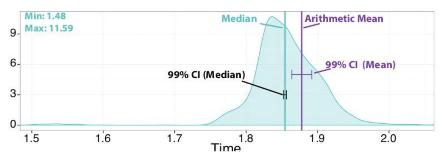
Reporting performance

Performance data is non-deterministic, so one run is not enough to correctly measure a program’s performance. That is because a program’s performance depends on the so-called noise:

• on a given compute node, other applications and/or the OS itself could interfere (scheduler, cache pollution…)
• across multiple nodes, there might be interferences on the network (ex. if two processes are trying to MPI_Send() to two different users’ processes, through the same physical link)

So, the correct solution is to run the application multiple times and report the entire distribution of timings.

“Friends Don’t Let Friends Make Bad Graphs” - a resource for data visualization

Runtime example: matrix-vector multiplication

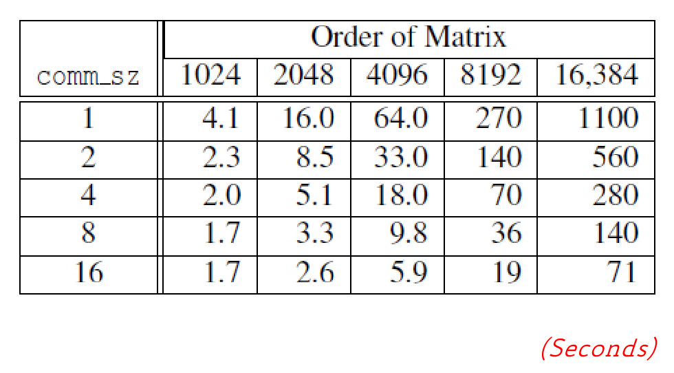
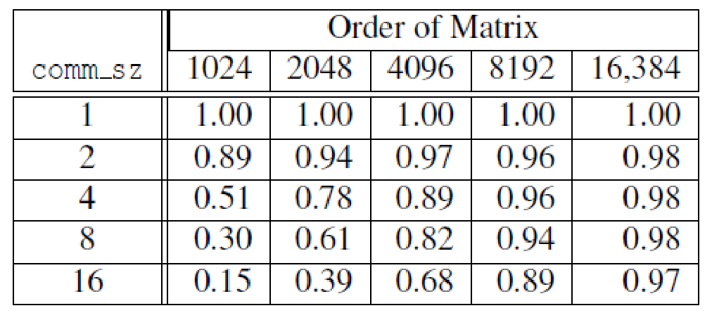
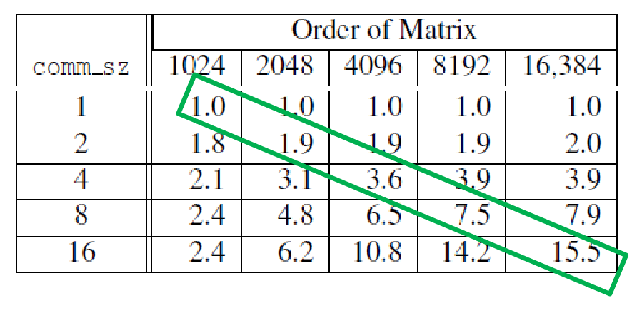
This is an example of different runtimes, depending on the matrices’ order and the number of processes used.

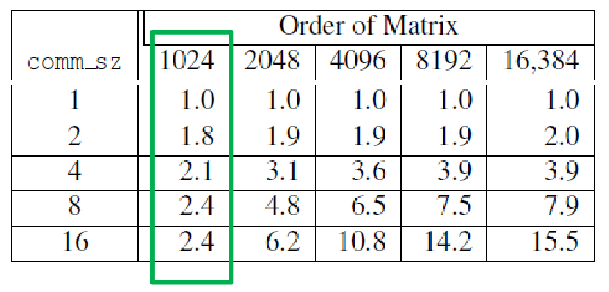
• we can see that, if the data is too small, it doesn’t make sense to use more processes, as the improvement in runtime could be marginal or even non-existent (as seen in 8, 1024 vs 16, 1024)

In general, the runtime increases with the problem size and decreases with the number of processes.

Expectations

Ideally, when running with $p$ processes, the program should be $p$ times faster than when running with 1 process. We define:

• $T_{serial}(n)$ as the time of our sequential application on a problem of size $n$ (e.g. the dimension of the matrix)
• $T_{parallel}(n,p)$ the time of our parallel application on a problem of size $n$, when running with $p$ processes
• $S(n,p)$ the speedup of our parallel application:

$$S(n,p)=\frac{T_{serial}(n)}{T_{parallel}(n,p)}$$

ideally, $S(n,p)=p$ (linear speedup)

the tests must be taken on the same type of cores/systems (i.e. one shouldn't compute the serial time on a CPU core and the parallel time on GPU cores)

what do we expect

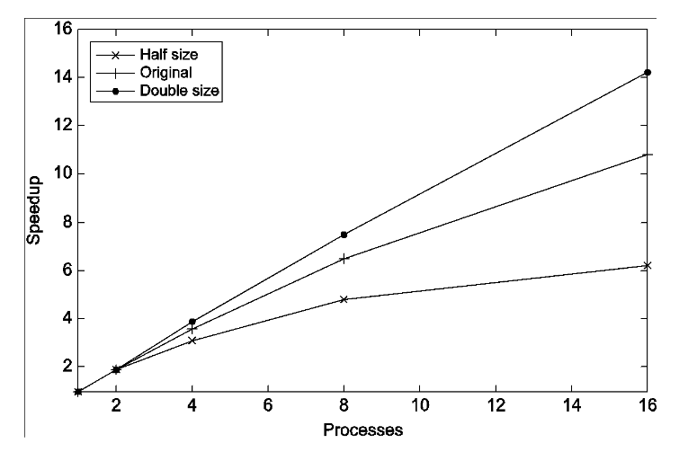
In general, we expect the speedup to get better when increasing the problem size $n$.

speedups of parallel matrix-vector multiplication

note !

Note that: $T_{serial}(n)\ne T_{parallel}(n,1)$

• the parallel and sequential implementations might be different, and in general, $T_{parallel}(n,1)\ge T_{serial}(n)$

We define scalability this way:

$S(n,p)=\frac{T_{parallel(n,1)}}{T_{parallel(n,p)}}$

• (measure of how well a program’s performance increases as more cores are added)

and (parallel) efficiency this way: $E(n,p)=\frac{S(n,p)}{p}=\frac{T_{serial}(n)}{p\times T_{parallel}(n,p)}$

• (measure of how effectively the processing resources are being used)

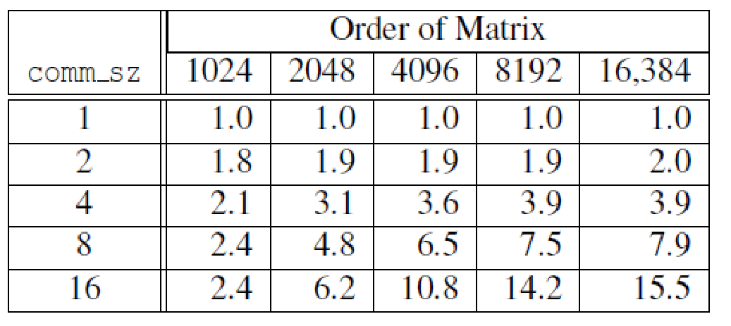
Ideally, we would like to have $E(n,p)=1$. In practice, it is $\le 1$, and it gets worse with smaller problems.

efficiency of parallel matrix-vector multiplication

strong vs weak scaling

Strong and weak scaling are two methods used to evaluate the scalability of a parallel program. They differ on whether the total problem size is kept fixed or scaled along with the processes.

• strong scaling ⟶ the problem size is fixed, the number of processes is increased
  • (if the efficiency stays high, the program is strong-scalable)
• weak scaling ⟶ the problem size is increased at the same rate as the number of processes
  • (if the efficiency stays high, the program is weak-scalable)

examples

The matrix-vector multiplication program is weak-scalable but not strong-scalable.

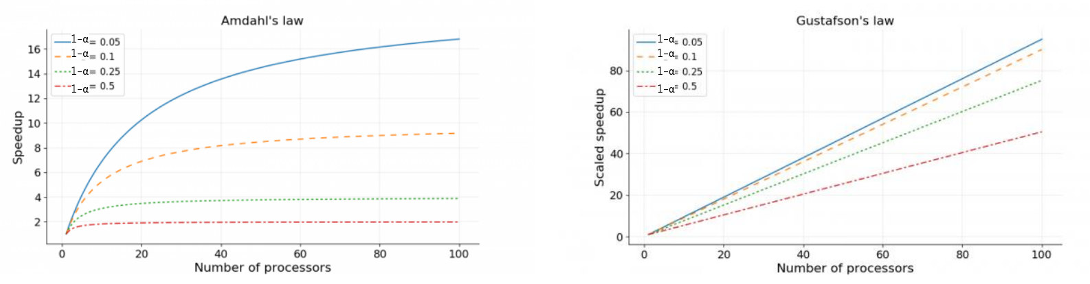
Amdahl’s law (strong scaling)

Idea

Every program has some part that cannot be parallelized (like reading/writing a file from disk, sending/receiving data over the network etc): serial fraction, $1-\alpha$

Amdahl’s law says that the speedup is limited by the serial fraction:

$$T_{\text{parallel}}(p)=(1-\alpha )T_{\text{serial}}+\alpha \frac{T_{\text{serial}}}{p}$$

The upper asymptotic limit of the speedup to which we can aim is

$$\underset{p\to \infty }{\lim }S(p)=\frac{1}{1-\alpha }$$

Gustafson’s law (weak scaling)

If we consider weak scaling, the parallel fraction increases with the problem size (i.e., the serial time remains constant, but the parallel time increases).

This is also known as scaled speedup.

$$S(n,p)=(1-\alpha )+\alpha p$$

Amdahl's law vs Gustafson's law